Quickstart Tutorial¶

galtab is a general approach for calculating the expectation value of counts-in-cells statistics for a given halo catalog and HOD model. It pretabulates placeholder galaxies inside each halo to yield rapid, deterministic results, which is ideal for MCMC likelihood evaluations.

This tutorial will demonstrate some basic Counts-in-Cylinders (CiC) calculations using the intended galtab workflow.

To cite galtab, learn more implementation details, and explore an example science use case, check out https://arxiv.org/abs/2309.08675.

Prerequisites¶

All of the following are pip installable

galtab
- numpy
- jax
- astropy
- halotools
matplotlib
jupyterlab

After installing the above and downloading the bolplanck z=0 halotools catalog, you should be able to run the following cell. In this cell:

set our cosmology and CiC parameters
choose an HOD model
load the simulation data

[1]:

import numpy as np
import matplotlib.pyplot as plt
import jax
from jax import numpy as jnp

from astropy import cosmology
import halotools.empirical_models as htem
import halotools.sim_manager as htsm
import halotools.mock_observables as htmo

import galtab

# Set our CiC parameters (all lengths are in Mpc/h)
proj_search_radius = 2.0
cylinder_half_length = 10.0
cic_edges = np.arange(-0.5, 16)

# Set our cosmology and HOD model
cosmo = cosmology.Planck13
hod = htem.PrebuiltHodModelFactory("zheng07", threshold=-21)

# Load Bolshoi-Planck simulation halos at z=0
halocat = htsm.CachedHaloCatalog(simname="bolplanck", redshift=0)
halocat.halo_table[:5]

[1]:

Table length=5

halo_vmax_firstacc	halo_dmvir_dt_tdyn	halo_macc	halo_scale_factor	halo_vmax_mpeak	halo_m_pe_behroozi	halo_delta_vmax_behroozi17	halo_xoff	halo_spin	halo_tidal_force	halo_scale_factor_firstacc	halo_c_to_a	halo_mvir_firstacc	halo_scale_factor_last_mm	halo_tidal_id	halo_scale_factor_mpeak	halo_pid	halo_m500c	halo_id	halo_halfmass_scale_factor	halo_upid	halo_t_by_u	halo_rvir	halo_vpeak	halo_dmvir_dt_100myr	halo_mpeak	halo_m_pe_diemer	halo_jx	halo_jy	halo_jz	halo_m2500c	halo_mvir	halo_voff	halo_axisA_z	halo_axisA_x	halo_axisA_y	halo_y	halo_b_to_a	halo_x	halo_z	halo_m200b	halo_vacc	halo_scale_factor_lastacc	halo_vmax	halo_m200c	halo_vx	halo_vy	halo_vz	halo_dmvir_dt_inst	halo_tidal_force_tdyn	halo_rs	halo_nfw_conc	halo_hostid	halo_mvir_host_halo
float32	float32	float32	float32	float32	float32	float32	float32	float32	float32	float32	float32	float32	float32	int64	float32	int64	float32	int64	float32	int64	float32	float32	float32	float32	float32	float32	float32	float32	float32	float32	float32	float32	float32	float32	float32	float32	float32	float32	float32	float32	float32	float32	float32	float32	float32	float32	float32	float32	float32	float32	float32	int64	float32
1001.57	12810.0	200800000000000.0	1.00231	1001.57	202700000000000.0	-0.0026	0.0257357	0.02391	0.11954	1.00231	0.47559	200800000000000.0	0.28343	2812606193	1.002	-1	116580000000000.0	2811042639	0.41506	-1	0.593	1.190447	1091.38	17390.0	200800000000000.0	111800000000000.0	2536000000000000.0	-474400000000000.0	-6566000000000000.0	65777000000000.0	200800000000000.0	21.34	19.2231	59.7891	-18.8001	43.14082	0.63663	36.17984	17.96339	223780000000000.0	1001.57	1.00231	1001.57	158240000000000.0	16.1	8.51	-78.88	17390.0	0.12244	0.137953	8.629367	2811042639	200800000000000.0
895.2	13760.0	179600000000000.0	1.00231	895.2	181000000000000.0	-0.01065	0.041987	0.06297	0.50587	1.00231	0.56181	179600000000000.0	0.29862	2811077105	1.002	-1	100360000000000.0	2811055606	0.50618	-1	0.627	1.146849	969.05	7324.0	179600000000000.0	128700000000000.0	1.074e+16	4931000000000000.0	-1.185e+16	47026000000000.0	179600000000000.0	41.91	41.2062	34.6803	17.8882	49.54417	0.8397	45.36644	40.01593	204460000000000.0	895.2	1.00231	895.2	142290000000000.0	2.46	264.77	-128.08	7324.0	0.491	0.185805	6.172326	2811055606	179600000000000.0
853.83	4666.0	129800000000000.0	1.00231	853.83	149500000000000.0	0.00531	0.026461901	0.03607	0.07568	1.00231	0.66381	129800000000000.0	0.49606	2810630242	1.002	-1	87766000000000.0	2809250167	0.491	-1	0.5774	1.029343	926.37	2747.0	129800000000000.0	80320000000000.0	2133000000000000.0	-3236000000000000.0	-3111000000000000.0	39496000000000.0	129800000000000.0	23.35	-17.5268	38.9596	24.3626	13.88261	0.76149	22.02318	9.80153	141210000000000.0	853.83	1.00231	853.83	112010000000000.0	18.49	124.89	-35.19	2747.0	0.10074	0.119293995	8.628624	2809250167	129800000000000.0
777.64	4401.0	103000000000000.0	1.00231	777.64	104800000000000.0	0.00498	0.0516998	0.05031	0.09677	1.00231	0.47302	103000000000000.0	0.38469	2820592816	1.002	-1	57781000000000.0	2809483946	0.65806	-1	0.6152	0.952978	831.17	2747.0	103000000000000.0	64200000000000.0	1713000000000000.0	-1488000000000000.0	4582000000000000.0	30529000000000.0	103000000000000.0	98.45	24.7744	-10.3568	38.9949	36.67881	0.7881	12.29788	34.18085	115110000000000.0	777.64	1.00231	777.64	82069000000000.0	-281.37	-115.39	-391.28	2747.0	0.10259	0.132334	7.201309	2809483946	103000000000000.0
748.56	11480.0	99470000000000.0	1.00231	748.56	107600000000000.0	0.05989	0.0779697	0.0348	0.12465	1.00231	0.47409	99470000000000.0	0.63275	2809483946	1.002	-1	59100000000000.0	2809272603	0.63781	-1	0.67	0.941893	748.56	5218.0	99470000000000.0	70970000000000.0	1207000000000000.0	-2126000000000000.0	-2677000000000000.0	26267000000000.0	99470000000000.0	118.79	29.2183	52.7796	6.18836	26.12877	0.66155	10.66037	22.5009	108110000000000.0	748.56	1.00231	748.56	84337000000000.0	-43.87	292.95	-171.47	5218.0	0.1579	0.14077	6.691006	2809272603	99470000000000.0

Calculate CiC the standard way with `halotools`¶

Populate the halocat with galaxies probabilistically from the HOD model
Compute the number of neighbors within a cylinder around each neighbor
Tally up a histogram of the neighbor counts for a given set of CiC bins

[2]:

# Choose your HOD parameters (in this case, we will keep them the same)
hod.param_dict.update({})

# Populated model galaxies and get their Cartesian coordinates
hod.populate_mock(halocat)
galaxies = hod.mock.galaxy_table
xyz = htmo.return_xyz_formatted_array(
    galaxies["x"], galaxies["y"], galaxies["z"], velocity=galaxies["vz"],
    velocity_distortion_dimension="z", period=halocat.Lbox, cosmology=cosmo
)

# Compute CiC (self-counting subtracted by the `-1`)
cic_counts = htmo.counts_in_cylinders(
    xyz, xyz, proj_search_radius, cylinder_half_length) - 1
cic_halotools = np.histogram(cic_counts, bins=cic_edges, density=True)[0]
cic_halotools

[2]:

array([0.3675878 , 0.25521013, 0.15238918, 0.08963731, 0.05152562,
       0.03218192, 0.0193437 , 0.01162925, 0.00420265, 0.00529649,
       0.00362694, 0.00270581, 0.00166955, 0.00149683, 0.00080599,
       0.00069085])

Now let’s do it the `galtab` way¶

[3]:

# Give the Tabulator the halo catalog and a fiducial HOD model
gtab = galtab.GalaxyTabulator(halocat, hod)

# Prepare the CICTabulator to make predictions
cictab = galtab.CICTabulator(gtab, proj_search_radius, cylinder_half_length,
                            bin_edges=cic_edges)

# Choose your HOD parameters (in this case, we will keep them the same)
hod.param_dict.update({})

# Predict CiC for this model
cic_galtab = cictab.predict(hod)
cic_galtab

WARNING:absl:No GPU/TPU found, falling back to CPU. (Set TF_CPP_MIN_LOG_LEVEL=0 and rerun for more info.)

[3]:

DeviceArray([0.35819536, 0.2572313 , 0.15485156, 0.09022042, 0.05297909,
             0.03188442, 0.01996169, 0.0124573 , 0.00806456, 0.00497749,
             0.00318336, 0.00215645, 0.0015641 , 0.00095675, 0.00078415,
             0.00053201], dtype=float32)

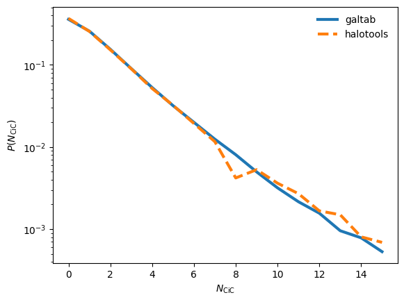
Plot the `galtab` vs. `halotools` comparison¶

galtab predicts the CiC expectation value (smooth + deterministic)
halotools draws a CiC realization (noisy + stochastic)

[4]:

cic_cens = 0.5 * (cic_edges[:-1] + cic_edges[1:])
plt.semilogy(cic_cens, cic_galtab, label="galtab", lw=3)
plt.semilogy(cic_cens, cic_halotools, label="halotools", lw=3, ls="--")
plt.legend(frameon=False)
plt.xlabel("$N_{\\rm CiC}$")
plt.ylabel("$P(N_{\\rm CiC})$")
plt.show()

In Development: Differentiate CiC w.r.t. the HOD parameter \(\log M_{\rm min}\)¶

galtab is implemented in JAX, so it is portable to GPU and differentiable (in principal), assuming your HOD model is compatible with JAX. Unfortunately, this requires a few modifications to halotools models. For example, let’s use the JaxZheng07Cens and JaxZheng07Sats models, originally implemented for the JaxTabCorr project.

We can construct a composite HOD model with our JAX-compatible mean occupation functions, which we call hod_jax. This model allows us to differentiate cictab.predict with jax.grad.

Note: You shouldn’t try using jax.jit directly on cictab.predict, since it contains some I/O lines that can’t be compiled. Rest assured that the primary expensive computations will automatically compile and run on the GPU if available.

[5]:

from galtab.jaxhalotools import JaxZheng07Cens, JaxZheng07Sats

# Create JAX-compatible composite HOD model
hod_jax = htem.HodModelFactory(
    centrals_occupation=JaxZheng07Cens(threshold=-21),
    satellites_occupation=JaxZheng07Sats(threshold=-21),
    centrals_profile=htem.TrivialPhaseSpace(),
    satellites_profile=htem.NFWPhaseSpace()
)

# Define function that predictions P(N_cic = 1)
def calc_cic1(logMmin=12.79):
    hod_jax.param_dict.update({"logMmin": logMmin})
    return cictab.predict(hod_jax, warn_p_over_1=False)[1]

# Define the derivative of calc_cic1
diff_cic1 = jax.grad(calc_cic1)

# Note that we shouldn't make logMmin too much lower than that of our fiducial
# model. If desired, make more conservative choices for the fiducial parameters.
# i.e., low logMmin / logM1 / logM0 values and large sigma_logM values
for logmmin in np.linspace(11.0, 15.0, 20):
    value = calc_cic1(logmmin)
    derivative = diff_cic1(logmmin)

    plt.plot(logmmin, value, "bo")
    plt.quiver(logmmin, value, 1, derivative, angles="xy")

plt.xlabel("$\\log M_{\\rm min}$")
plt.ylabel("$P(N_{\\rm CiC} = 1)$")
plt.show()

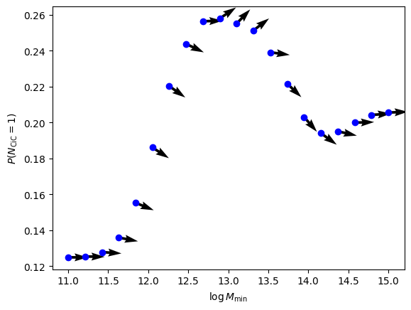
`jax.grad` (the arrows in the above plot) isn’t working yet…¶

I actually wasn’t expecting the above to work perfectly, because it’s using the Monte-Carlo mode, which isn’t perfectly continuous
But analytic mode moment derivatives aren’t working either…
TODO: Figure out what’s going wrong

Quickstart Tutorial¶

Prerequisites¶

Calculate CiC the standard way with `halotools`¶

Now let’s do it the `galtab` way¶

Plot the `galtab` vs. `halotools` comparison¶

In Development: Differentiate CiC w.r.t. the HOD parameter \(\log M_{\rm min}\)¶

`jax.grad` (the arrows in the above plot) isn’t working yet…¶

Table of Contents

Previous topic

Next topic

This Page

Quickstart Tutorial¶

Prerequisites¶

Calculate CiC the standard way with halotools¶

Now let’s do it the galtab way¶

Plot the galtab vs. halotools comparison¶

In Development: Differentiate CiC w.r.t. the HOD parameter \(\log M_{\rm min}\)¶

jax.grad (the arrows in the above plot) isn’t working yet…¶

Calculate CiC the standard way with `halotools`¶

Now let’s do it the `galtab` way¶

Plot the `galtab` vs. `halotools` comparison¶

`jax.grad` (the arrows in the above plot) isn’t working yet…¶