Quickstart Tutorial

galtab is a general approach for calculating the expectation value of counts-in-cells statistics for a given halo catalog and HOD model. It pretabulates placeholder galaxies inside each halo to yield rapid, deterministic results, which is ideal for MCMC likelihood evaluations.

This tutorial will demonstrate some basic Counts-in-Cylinders (CiC) calculations using the intended galtab workflow.

To cite galtab, learn more implementation details, and explore an example science use case, check out https://arxiv.org/abs/2309.08675.

Prerequisites

All of the following are pip installable

• galtab

  • numpy

  • jax

  • astropy

  • halotools

• matplotlib

• jupyterlab

After installing the above and downloading the bolplanck z=0 halotools catalog, you should be able to run the following cell. In this cell:

• set our cosmology and CiC parameters

• choose an HOD model

• load the simulation data

import numpy as np
import matplotlib.pyplot as plt
import jax

from astropy import cosmology
import halotools.empirical_models as htem
import halotools.sim_manager as htsm
import halotools.mock_observables as htmo

import galtab

# Download an example halotools catalog
htsm.DownloadManager().download_processed_halo_table(
    'bolplanck', 'rockstar', 0.0)

... Downloading data from the following location:
http://www.astro.yale.edu/aphearin/Data_files/halo_catalogs/bolplanck/rockstar/hlist_1.00231.list.halotools_v0p4.hdf5

 ... Saving the data with the following filename:
/home/docs/.astropy/cache/halotools/halo_catalogs/bolplanck/rockstar/hlist_1.00231.list.halotools_v0p4.hdf5

5% complete, elapsed time = 1 seconds
10% complete, elapsed time = 1 seconds
15% complete, elapsed time = 2 seconds
20% complete, elapsed time = 2 seconds
25% complete, elapsed time = 3 seconds
30% complete, elapsed time = 3 seconds
35% complete, elapsed time = 3 seconds
40% complete, elapsed time = 4 seconds
45% complete, elapsed time = 4 seconds
50% complete, elapsed time = 5 seconds
55% complete, elapsed time = 5 seconds
60% complete, elapsed time = 6 seconds
65% complete, elapsed time = 6 seconds
70% complete, elapsed time = 7 seconds
75% complete, elapsed time = 7 seconds
80% complete, elapsed time = 8 seconds
85% complete, elapsed time = 8 seconds
90% complete, elapsed time = 8 seconds
95% complete, elapsed time = 9 seconds
100% complete, elapsed time = 9 seconds

Total runtime to download pre-processed halo catalog = 9.4 seconds


The halo catalog has been successfully downloaded to the following location:
/home/docs/.astropy/cache/halotools/halo_catalogs/bolplanck/rockstar/hlist_1.00231.list.halotools_v0p4.hdf5

This filename and its associated metadata have also been added to the Halotools cache log,
as reflected by a newly added line to the following ASCII file:

/home/docs/.astropy/cache/halotools/halo_table_cache_log.txt

Since the catalog will now be recognized in cache,
you can load it into memory using the following syntax:

>>> from halotools.sim_manager import CachedHaloCatalog
>>> halocat = CachedHaloCatalog(simname = 'bolplanck', halo_finder = 'rockstar', version_name = 'halotools_v0p4', redshift = -0.0023)

For convenience, you can set this catalog to be your default catalog
and omit the CachedHaloCatalog constructor arguments.
To do that, change the following variables in the
halotools.sim_manager.sim_defaults module:
``default_simname``, ``default_halo_finder``, ``default_version_name`` and ``default_redshift``.

Tabular data storing the actual halos is bound to the ``halo_table``
attribute of ``halocat`` in the form of an Astropy Table:

>>> halos = halocat.halo_table

Halo properties are accessed in the same manner as a python dictionary or Numpy structured array:

>>> mass_array = halos['halo_mvir']

The ``halocat`` object also contains additional metadata
such as ``halocat.simname``, ``halocat.redshift`` and ``halocat.fname``
that you can use for sanity checks on your bookkeeping.

Note that if you move this halo catalog into a new location on disk,
you must update both the ``fname`` metadata of the hdf5 file
as well as the``fname`` column of the corresponding entry in the log.
You can accomplish this with the ``update_cached_file_location``method
of the HaloTableCache class.

# Set our CiC parameters (all lengths are in Mpc/h)
proj_search_radius = 2.0
cylinder_half_length = 10.0
cic_edges = np.arange(-0.5, 16)

# Set our cosmology and HOD model
cosmo = cosmology.Planck13
hod = htem.PrebuiltHodModelFactory("zheng07", threshold=-21)

# Load Bolshoi-Planck simulation halos at z=0
halocat = htsm.CachedHaloCatalog(simname="bolplanck", redshift=0)
halocat.halo_table[:5]

Table length=5

halo_vmax_firstacc	halo_dmvir_dt_tdyn	halo_macc	halo_scale_factor	halo_vmax_mpeak	halo_m_pe_behroozi	halo_delta_vmax_behroozi17	halo_xoff	halo_spin	halo_tidal_force	halo_scale_factor_firstacc	halo_c_to_a	halo_mvir_firstacc	halo_scale_factor_last_mm	halo_tidal_id	halo_scale_factor_mpeak	halo_pid	halo_m500c	halo_id	halo_halfmass_scale_factor	halo_upid	halo_t_by_u	halo_rvir	halo_vpeak	halo_dmvir_dt_100myr	halo_mpeak	halo_m_pe_diemer	halo_jx	halo_jy	halo_jz	halo_m2500c	halo_mvir	halo_voff	halo_axisA_z	halo_axisA_x	halo_axisA_y	halo_y	halo_b_to_a	halo_x	halo_z	halo_m200b	halo_vacc	halo_scale_factor_lastacc	halo_vmax	halo_m200c	halo_vx	halo_vy	halo_vz	halo_dmvir_dt_inst	halo_tidal_force_tdyn	halo_rs	halo_nfw_conc	halo_hostid	halo_mvir_host_halo
float32	float32	float32	float32	float32	float32	float32	float32	float32	float32	float32	float32	float32	float32	int64	float32	int64	float32	int64	float32	int64	float32	float32	float32	float32	float32	float32	float32	float32	float32	float32	float32	float32	float32	float32	float32	float32	float32	float32	float32	float32	float32	float32	float32	float32	float32	float32	float32	float32	float32	float32	float32	int64	float32
1001.57	12810.0	200800000000000.0	1.00231	1001.57	202700000000000.0	-0.0026	0.0257357	0.02391	0.11954	1.00231	0.47559	200800000000000.0	0.28343	2812606193	1.002	-1	116580000000000.0	2811042639	0.41506	-1	0.593	1.190447	1091.38	17390.0	200800000000000.0	111800000000000.0	2536000000000000.0	-474400000000000.0	-6566000000000000.0	65777000000000.0	200800000000000.0	21.34	19.2231	59.7891	-18.8001	43.14082	0.63663	36.17984	17.96339	223780000000000.0	1001.57	1.00231	1001.57	158240000000000.0	16.1	8.51	-78.88	17390.0	0.12244	0.137953	8.629367	2811042639	200800000000000.0
895.2	13760.0	179600000000000.0	1.00231	895.2	181000000000000.0	-0.01065	0.041987	0.06297	0.50587	1.00231	0.56181	179600000000000.0	0.29862	2811077105	1.002	-1	100360000000000.0	2811055606	0.50618	-1	0.627	1.146849	969.05	7324.0	179600000000000.0	128700000000000.0	1.074e+16	4931000000000000.0	-1.185e+16	47026000000000.0	179600000000000.0	41.91	41.2062	34.6803	17.8882	49.54417	0.8397	45.36644	40.01593	204460000000000.0	895.2	1.00231	895.2	142290000000000.0	2.46	264.77	-128.08	7324.0	0.491	0.185805	6.172326	2811055606	179600000000000.0
853.83	4666.0	129800000000000.0	1.00231	853.83	149500000000000.0	0.00531	0.026461901	0.03607	0.07568	1.00231	0.66381	129800000000000.0	0.49606	2810630242	1.002	-1	87766000000000.0	2809250167	0.491	-1	0.5774	1.029343	926.37	2747.0	129800000000000.0	80320000000000.0	2133000000000000.0	-3236000000000000.0	-3111000000000000.0	39496000000000.0	129800000000000.0	23.35	-17.5268	38.9596	24.3626	13.88261	0.76149	22.02318	9.80153	141210000000000.0	853.83	1.00231	853.83	112010000000000.0	18.49	124.89	-35.19	2747.0	0.10074	0.119293995	8.628624	2809250167	129800000000000.0
777.64	4401.0	103000000000000.0	1.00231	777.64	104800000000000.0	0.00498	0.0516998	0.05031	0.09677	1.00231	0.47302	103000000000000.0	0.38469	2820592816	1.002	-1	57781000000000.0	2809483946	0.65806	-1	0.6152	0.952978	831.17	2747.0	103000000000000.0	64200000000000.0	1713000000000000.0	-1488000000000000.0	4582000000000000.0	30529000000000.0	103000000000000.0	98.45	24.7744	-10.3568	38.9949	36.67881	0.7881	12.29788	34.18085	115110000000000.0	777.64	1.00231	777.64	82069000000000.0	-281.37	-115.39	-391.28	2747.0	0.10259	0.132334	7.201309	2809483946	103000000000000.0
748.56	11480.0	99470000000000.0	1.00231	748.56	107600000000000.0	0.05989	0.0779697	0.0348	0.12465	1.00231	0.47409	99470000000000.0	0.63275	2809483946	1.002	-1	59100000000000.0	2809272603	0.63781	-1	0.67	0.941893	748.56	5218.0	99470000000000.0	70970000000000.0	1207000000000000.0	-2126000000000000.0	-2677000000000000.0	26267000000000.0	99470000000000.0	118.79	29.2183	52.7796	6.18836	26.12877	0.66155	10.66037	22.5009	108110000000000.0	748.56	1.00231	748.56	84337000000000.0	-43.87	292.95	-171.47	5218.0	0.1579	0.14077	6.691006	2809272603	99470000000000.0

Calculate CiC the standard way with halotools

• Populate the halocat with galaxies probabilistically from the HOD model

• Compute the number of neighbors within a cylinder around each neighbor

• Tally up a histogram of the neighbor counts for a given set of CiC bins

# Choose your HOD parameters (in this case, we will keep them the same)
hod.param_dict.update({})

# Populated model galaxies and get their Cartesian coordinates
hod.populate_mock(halocat, seed=0)
galaxies = hod.mock.galaxy_table
xyz = htmo.return_xyz_formatted_array(
    galaxies["x"], galaxies["y"], galaxies["z"], velocity=galaxies["vz"],
    velocity_distortion_dimension="z", period=halocat.Lbox, cosmology=cosmo
)

# Compute CiC (self-counting subtracted by the `-1`)
cic_counts = htmo.counts_in_cylinders(
    xyz, xyz, proj_search_radius, cylinder_half_length,
    period=halocat.Lbox) - 1
cic_halotools = np.histogram(cic_counts, bins=cic_edges, density=True)[0]
cic_halotools

array([0.35818234, 0.24693701, 0.15634167, 0.09105551, 0.05619787,
       0.03474259, 0.0190394 , 0.01392005, 0.01035375, 0.00500431,
       0.00270348, 0.00155306, 0.00126546, 0.0013805 , 0.00063273,
       0.00069025])

Now let’s do it the galtab way

# Give the Tabulator the halo catalog and a fiducial HOD model
gtab = galtab.GalaxyTabulator(halocat, hod)

# Prepare the CICTabulator to make predictions
cictab = galtab.CICTabulator(gtab, proj_search_radius, cylinder_half_length,
                            bin_edges=cic_edges)

# Choose your HOD parameters (in this case, we will keep them the same)
hod.param_dict.update({})

# Predict CiC for this model
cic_galtab = cictab.predict(hod)
cic_galtab

Array([0.35875157, 0.25464624, 0.15486689, 0.09135279, 0.05421961,
       0.03248107, 0.01915211, 0.01244971, 0.00771107, 0.00501356,
       0.0033694 , 0.00225268, 0.00150615, 0.00102266, 0.00068709,
       0.00051736], dtype=float32)

Optionally, write the CIC tabulation to disk for later use:

# Pickle the CICTabulator - creates a large file named `cictab.pickle`:
cictab.save("cictab.pickle")

# And load it back with:
cictab = galtab.CICTabulator.load("cictab.pickle")
gtab = cictab.galtabulator

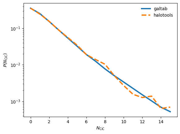
Plot the galtab vs. halotools comparison

• galtab predicts the CiC expectation value (smooth + deterministic)

• halotools draws a CiC realization (noisy + stochastic)

cic_cens = 0.5 * (cic_edges[:-1] + cic_edges[1:])
plt.semilogy(cic_cens, cic_galtab, label="galtab", lw=3)
plt.semilogy(cic_cens, cic_halotools, label="halotools", lw=3, ls="--")
plt.legend(frameon=False)
plt.xlabel("$N_{\\rm CiC}$")
plt.ylabel("$P(N_{\\rm CiC})$")
plt.show()

In Development: Differentiate CiC w.r.t. the HOD parameter \(\log M_{\rm min}\)

galtab is implemented in JAX, so it is portable to GPU and differentiable (in principal), assuming your HOD model is compatible with JAX. Unfortunately, this requires a few modifications to halotools models. For example, let’s use the JaxZheng07Cens and JaxZheng07Sats models, originally implemented for the JaxTabCorr project.

We can construct a composite HOD model with our JAX-compatible mean occupation functions, which we call hod_jax. This model allows us to differentiate cictab.predict with jax.grad.

Note: You shouldn’t try using jax.jit directly on cictab.predict, since it contains some lines of code that can’t be compiled. Rest assured that the primary expensive computations will automatically compile and run on the GPU if available.

from galtab.jaxhalotools import JaxZheng07Cens, JaxZheng07Sats

# Create JAX-compatible composite HOD model
def make_hod_jax():
    return htem.HodModelFactory(
        centrals_occupation=JaxZheng07Cens(threshold=-21),
        satellites_occupation=JaxZheng07Sats(threshold=-21),
        centrals_profile=htem.TrivialPhaseSpace(),
        satellites_profile=htem.NFWPhaseSpace()
    )

# Define function that predictions P(N_cic = 1)
def calc_cic1(logMmin=12.79):
    hod_jax = make_hod_jax()
    hod_jax.param_dict.update({"logMmin": logMmin})
    return cictab.predict(hod_jax, warn_p_over_1=False)[1]

# Define the derivative of calc_cic1
diff_cic1 = jax.grad(calc_cic1)

# Note that we shouldn't make logMmin too much lower than that of our fiducial
# model. If desired, make more conservative choices for the fiducial parameters.
# i.e., low logMmin / logM1 / logM0 values and large sigma_logM values
for logmmin in np.linspace(11.0, 15.0, 20):
    value = calc_cic1(logmmin)
    derivative = diff_cic1(logmmin)

    plt.plot(logmmin, value, "bo")
    plt.quiver(logmmin, value, 1, derivative, angles="xy")

plt.xlabel("$\\log M_{\\rm min}$")
plt.ylabel("$P(N_{\\rm CiC} = 1)$")
plt.show()

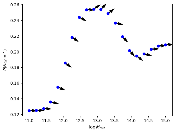
jax.grad (the arrows in the above plot) isn’t working yet…

• I actually wasn’t expecting the above to work perfectly, because it’s using the Monte-Carlo mode, which isn’t perfectly continuous

• But analytic mode moment derivatives aren’t working either…

• TODO: Figure out what’s going wrong